User Guide-Supported ISP algorithms

PVA ISP for
NVIDIA Jetson

Table of Contents [Sticky]

Introduction

This page explains the algorithms implemented in PVA ISP and how they are configured in params.yaml.

The below-mentioned information applies to both the C++ application and GStreamer.

Supported ISP Algorithms

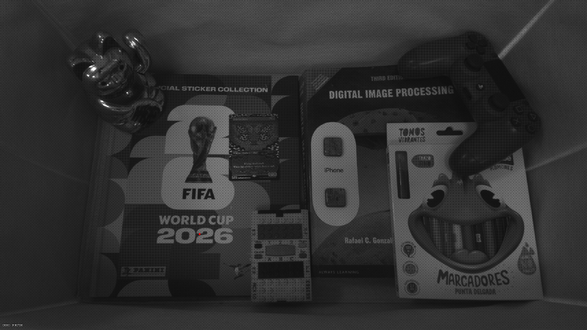Input Bayer image
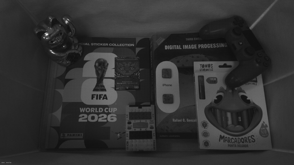Decompanding
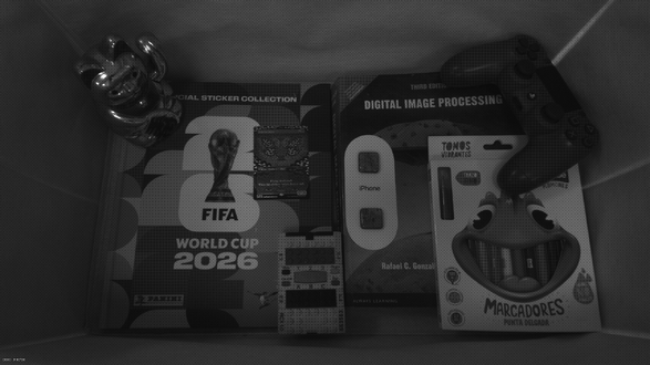Black level correction
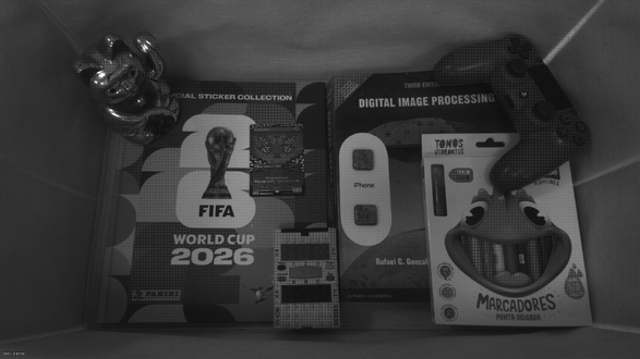Auto white balance
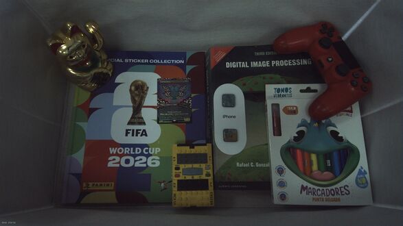Demosaicing
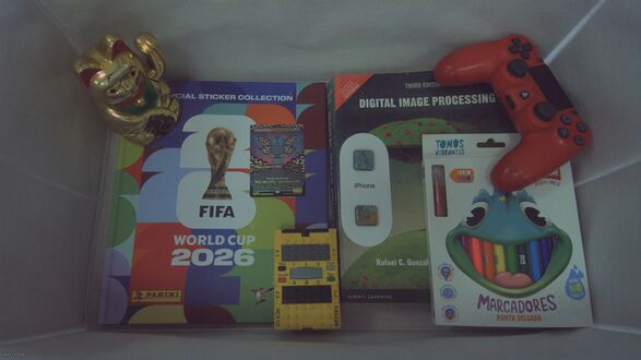Global tone mapping
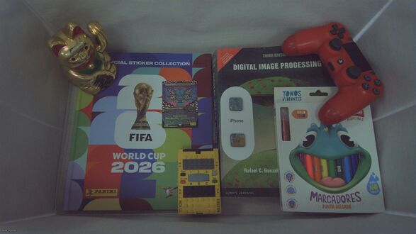Gamma tone mapping
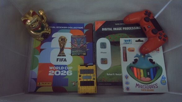NV12 output

PVA ISP provides a collection of image processing algorithms that can be combined to build custom ISP pipelines.

Each algorithm is implemented as an independent processing stage that can be executed individually or connected with other stages to form complete image processing workflows.

The current implementation supports the following ISP stages:

Algorithm	Input Format	Output Format	Supported Bit Depth
Decompanding	Bayer RAW	Bayer RAW	Input: 10/12/14-bit Output: 16-bit
Black Level Correction	Bayer RAW	Bayer RAW	16-bit
Histogram Generation	Bayer RAW	Histogram Statistics	16-bit Bayer input
White Balance	Bayer RAW	Bayer RAW	16-bit
Demosaicing	Bayer RAW	RGB	Input: 16-bit Bayer Output: 16-bit RGB
Global Tone Mapping	RGB	RGB	Input: 16-bit RGB Output: 8-bit RGB
Gamma Tone Mapping	RGB	RGB	8-bit RGB
NV12 Conversion	RGB	NV12	Input: 8-bit RGB Output: 8-bit NV12

Configuration Model

The configuration YAML file is organized by algorithm:

decompand
convolution
black_level
digital_gain
white_balance
demosaic
histogram
auto_exposure
gamma_tone_mapping
global_tone_mapping
debug

The loader applies a schema rule and also enforces a few runtime-only constraints:

decompand.x_pts and decompand.y_pts must have the same length
both decompand point lists must be strictly increasing
global_tone_mapping.gtm_scale_min <= gtm_scale_max
auto_exposure.min_exposure <= max_exposure
auto_exposure.min_gain <= max_gain

An example params.yml is collapsed below:

Example: params.yaml

# yaml-language-server: $schema=./params.schema.yaml
# Copyright (C) 2026 RidgeRun, LLC (http://www.ridgerun.com)
# All Rights Reserved.
#
# The contents of this software are proprietary and confidential to RidgeRun,
# LLC.  No part of this program may be photocopied, reproduced or translated
# into another programming language without prior written consent of
# RidgeRun, LLC.  The user is free to modify the source code after obtaining
# a software license from RidgeRun.  All source code changes must be provided
# back to RidgeRun without any encumbrance.

# Reference parameter file for the ISP examples.
# This sample matches `params.schema.yaml` and the runtime loader used by:
# - isp_minimal
# - isp_minimal_cuda
# - isp_app

decompand:
  input_shift: 4
  x_pts: [0, 1107, 3325, 7766, 16652, 34430, 52207, 56648, 65535]
  y_pts: [0, 1098, 1885, 2501, 3062, 3602, 3914, 3975, 4095]

convolution:
  kernel: [1, 2, 1, 2, 4, 2, 1, 2, 1]
  shift: 4

black_level:
  channel00: 16
  channel01: 16
  channel10: 16
  channel11: 16

digital_gain:
  gain: 1.5

white_balance:
  u_ref: [0.982, 0.789, 0.668, 0.558, 0.426]
  v_ref: [0.308, 0.382, 0.445, 0.428, 0.678]
  use_calibration: false
  manual_wb: false
  manual_wb_gains: [1.0, 1.0, 1.0]

demosaic:
  bayer_pattern: 0

histogram:
  bit_depth: 16
  use_mask: false

auto_exposure:
  kp_exposure: 40.0
  ki_exposure: 1.0
  kd_exposure: 8.0
  kp_gain: 5000000.0
  ki_gain: 10.0
  kd_gain: 500.0
  reference_mean: 120.0
  dynamic_range: 255.0
  min_exposure: 5000
  max_exposure: 20000
  min_gain: 2000000
  max_gain: 100000000
  camera_index: 0
  enable_v4l2: false

gamma_tone_mapping:
  gamma: 2.2

global_tone_mapping:
  brightness: 0.18
  gtm_scale_min: 0.0001
  gtm_scale_max: 0.01
  gtm_temporal_alpha: 1.0
  saturation: 1.0

debug:
  export_scene_key: false
  export_debug_csv: false
  debug_export_frame_index: 0

Decompanding

Many image sensors apply a non-linear response curve to better distribute code values across the available dynamic range. Decompanding reverses that compression by applying a piecewise linear (PWL) mapping defined by configuration points, producing output values that are closer to a linear light representation.

In this stage, the decompanding points are not an additional image input. Instead, they act as control parameters that define the PWL transfer function applied to each incoming pixel.

In the plot, the horizontal axis represents the compressed sensor input code values, while the vertical axis represents the expanded output values used internally by the ISP. Changes in slope across the curve reflect how the sensor compresses different regions of the dynamic range and how the ISP reconstructs them for later processing.

The stage builds a piecewise linear lookup table from the control points in the YAML file.

Parameter	Default in `params.yaml`	Effect
`input_shift`	`4`	Right-shifts the input samples before the LUT lookup to delete any padding. This adapts the decompand curve to packed RAW formats and discards low-order bits that are not part of the effective sample.
`x_pts`	`[0, 1107, 3325, 7766, 16652, 34430, 52207, 56648, 65535]`	Output-domain control points for the piecewise curve.
`y_pts`	`[0, 1098, 1885, 2501, 3062, 3602, 3914, 3975, 4095]`	Input-domain control points for the piecewise curve. These define the transfer function uploaded to the decompand kernel.

Important details:

The first point must be 0 for both arrays.
Both lists must be strictly increasing.
The runtime implementation uses these points to build the stage-owned VLUT before processing starts.

Typical Use Cases:

High dynamic range sensors
Non-linear sensor output formats

You can find more about this algorithm stage by visiting Decompand Stage

Black Level Correction

The Black Level Correction (BLC) stage removes sensor black offsets and establishes a proper black reference level.

This stage is typically one of the first operations performed after image acquisition. The goal of black leveling is to recover a signal proportional to the actual light intensity:

x_corrected ≈ x_signal

This is achieved by removing the offset B. Black leveling uses optical black pixels (shielded with opaque material) to estimate average black level value, in Bayer-pattern sensors (e.g., BGGR), each color channel has a different offset, but the simplest correction for each channel is:

x_corrected = x_signal - B

After black level correction, the sensor signal can be modeled as:

x_corrected = S · L + n

where:

L: scene illumination
S: sensor sensitivity
n: noise

At this stage, the signal is linear but may not have the desired exposure level. Digital gain is used to scale the signal in order to adjust brightness:

y = g · x_corrected

where:

g: digital gain factor

Unlike analog gain, digital gain does not improve signal quality. Applying gain:

y = g(S · L + n)

This implies:

Signal is amplified
Noise is also amplified

Digital gain acts as a post-capture exposure adjustment.

Parameter	Default in `params.yaml`	Effect
`channel00`	`16`	Optical-black offset for pixels at even row/even column.
`channel01`	`16`	Optical-black offset for pixels at even row/odd column.
`channel10`	`16`	Optical-black offset for pixels at odd row/even column.
`channel11`	`16`	Optical-black offset for pixels at odd row/odd column.
`digital_gain.gain`	`1.5`	Multiplies the correction factors used after optical-black subtraction. This is a global RAW-domain boost applied in fixed point.

Implementation notes:

The stage computes a correction factor per Bayer site from the optical-black value.
Those factors are converted to Q7 fixed-point values before being uploaded to the kernel.
The correction is applied before later stages such as white balance and demosaic.

Sites:

You can learn more about black level correction stage by visiting: Black Level Stage

Histogram Generation

The histogram stage computes image statistics directly from Bayer-domain image data.

Histograms can be used for image analysis, exposure estimation, tuning workflows, and validation.

Parameter	Default in `params.yaml`	Effect
`bit_depth`	`16`	Logical bit depth used to map decompanded samples into histogram bins. The implementation uses this to determine the bin shift before accumulation.
`use_mask`	`false`	Enables or disables use of the histogram mask.

Notes:

The YAML sample does not include a mask file path.
The example applications can load an external histogram mask and pass it to the stage as runtime data.
If no mask is provided, the stage uses a uniform mask.
The histogram output is the input to Auto Exposure.

Typical Use Cases :

Exposure analysis
Image characterization
ISP tuning workflows

You can learn more about the stage by visiting: Histogram Stage

White Balance

Its primary purpose is to ensure that white objects appear white, regardless of the light source. This, in turn, ensures that all other colors are also rendered accurately. Without proper white balance, these color casts can distort the color accuracy in embedded vision cameras.
White balance adjustments correct these color imbalances by shifting the colors in the image so that white appears white and other colors appear natural.
So basically white balance compensates for illumination by applying per-channel gains:

R' = g_R · R  
G' = g_G · G  
B' = g_B · B

The white balance stage can be understood as a three-step process:

Estimate the global or local color of the scene
Compute correction gains per channel
Apply the gains to every pixel

You can find more information about this stage by visiting:Auto white balance stage

The gains can be automatically computed based on chromaticity reference points or manually set.

Parameter	Default in `params.yaml`	Effect
`u_ref`	`[0.982, 0.789, 0.668, 0.558, 0.426]`	Five U-axis chromaticity reference points used to shape the calibration-based gain computation.
`v_ref`	`[0.308, 0.382, 0.445, 0.428, 0.678]`	Five V-axis chromaticity reference points used together with `u_ref`.
`use_calibration`	`false`	Selects the calibration-weighted path for gain generation.
`manual_wb`	`false`	Switches the final white-balance stage to manual gains instead of consuming the generated gain stream.
`manual_wb_gains`	`[1.0, 1.0, 1.0]`	Manual RGB gains used when `manual_wb` is enabled.

How it works:

If manual_wb is false, the pipeline can consume a generated gains frame.
If use_calibration is true, that gain generation uses the calibration references from u_ref and v_ref.
The gain-generation stage is implemented separately from the final white-balance multiplier so graphs can include or skip Black Level Correction.

Demosaicing

The purpose of demosaicing is to reconstruct a full RGB value for every pixel location. For each pixel, the two missing channels must be estimated from neighboring samples:

(R(x,y), G(x,y), B(x,y))

This reconstruction step is necessary before later ISP stages such as tone mapping, color correction, or gamma processing can operate correctly.

In the Bayer pattern, a pixel contains only a red value, and the missing green and blue values could be estimated by averaging nearby green and blue pixels. This basic approach is known as bilinear interpolation. It works reasonably well in smooth image regions, but it tends to blur edges and generate visible artifacts around fine detail.

The main difficulty comes from edges and textures. If interpolation is performed across an edge instead of along it, the reconstructed image may contain false colors, zipper-like patterns, or loss of sharpness. Because of this, practical demosaicing algorithms try to use local image structure to guide the interpolation process.

PVA ISP currently implements a Bayer-to-RGB demosaicing algorithm based on the Malvar-He-Cutler approach. This method starts from bilinear interpolation and adds correction terms that improve edge reconstruction. The idea is that neighboring color channels are strongly correlated in natural images. Instead of reconstructing each channel independently, the algorithm uses differences between channels to refine the estimate.

For example, consider a red pixel where the green value is missing. A simple estimate of green can be obtained from the surrounding green samples:

G_interp = (G_up + G_down + G_left + G_right) / 4

However, this estimate alone ignores local structure. The Malvar-He-Cutler method improves it by adding a correction term derived from nearby red values:

G = G_interp + α (R_center - R_avg)

where:

R_center is the red value at the current pixel
R_avg is the average of neighboring red pixels
α is a constant coefficient defined by the demosaicing filter design

In the practical implementation, this correction is not applied as a separate runtime parameter. Instead, it is incorporated into the convolution kernel coefficients used for each reconstruction case.

The correction acts similarly to a Laplacian or high-frequency enhancement term. If the local region contains an edge, the correction helps preserve it instead of smoothing it away.

In practice, the reconstruction is implemented using convolution filters. The missing channel at each location is computed by applying a kernel over a neighborhood:

C_out(x,y) = Σ w(i,j) · I(x+i, y+j)

In this expression, each neighboring sample is multiplied by its corresponding kernel coefficient first, and the final pixel value is obtained by summing all those products. In other words, this is a weighted sum over the local neighborhood. The filter coefficients depend on both:

the Bayer position of the current pixel
the channel being reconstructed

This means that different kernels are used for different interpolation cases.

Figure 5. Input and outputs Demosaicing algorithm.

The demosaic can be controlled using the following table:

Parameter	Default in `params.yaml`	Effect
`bayer_pattern`	`0`	Selects the Bayer mosaic ordering. The schema allows `0` to `3`, which map to `BGGR`, `RGGB`, `GBRG`, and `GRBG`.

Implementation notes:

The stage reconstructs planar RGB16 output.
In some graphs it also computes a scene-key side output. That behavior is controlled by the pipeline, not by the YAML file.
The scene-key path is used when Global Tone Mapping needs the statistics directly from Demosaic.

You can learn more about this stage by visiting: Demosaic Stage

Convolution

The convolution algorithm applies a configurable 3x3 filter independently to each RGB channel of the input image. The implementation is optimized for execution on the NVIDIA PVA and processes the image tile by tile using vector instructions.

The kernel coefficients are configurable, allowing the same algorithm to implement different filtering operations such as smoothing, sharpening, or edge enhancement.

The algorithm performs exactly the same convolution independently on each color plane.

Input RGB
Red   → 3×3 Convolution → Filtered Red
Green → 3×3 Convolution → Filtered Green
Blue  → 3×3 Convolution → Filtered Blue

No interaction exists between color channels during the convolution itself.

An implementation detail, the algorithm divides the image into fixed-size tiles. Each tile contains 64x64 pixels. Thus, to correctly evaluate pixels located at tile boundaries, an additional one-pixel halo is included around every tile. This provides the neighboring pixels required by the 3x3 filter while allowing every tile to be processed independently.

Moreover, the implementation is heavily vectorized for the PVA architecture. Rather than processing one pixel at a time, multiple pixels are processed simultaneously using vector instructions.

After the convolution accumulation is complete, the result is shifted by a configurable number of bits.

Filtered Pixel = Accumulated Sum >> Shift

The shift is used to normalize the accumulated value according to the kernel gain. Finally, the output is saturated to the valid 16-bit unsigned range.

The configuration options are presented below:

Parameter	Default in `params.yaml`	Effect
`kernel`	`[1, 2, 1, 2, 4, 2, 1, 2, 1]`	Nine signed coefficients in row-major order for the 3x3 filter.
`shift`	`4`	Right-shift applied after convolution.

Notes:

The kernel is packed into the PVA command program during configuration.
The scene-key output is built from the filtered RGB data and is consumed by Global Tone Mapping.

For more information, visit the Convolution stage.

Global Tone Mapping

Global tone mapping is used to compress the dynamic range of an image so it can be displayed correctly on standard screens. Images coming from the sensor or previous stages may contain a very wide range of luminance values. Some regions can be extremely bright, while others are very dark. However, display devices can only represent a limited range of values. Because of this, the image needs to be remapped so that both dark and bright regions remain visible at the same time.

The algorithm operates in a few simple steps. First, the image is converted to luminance. Instead of working directly on RGB values, the algorithm extracts a single brightness value per pixel. This makes it easier to control the overall intensity of the image without affecting color ratios. Then, a global measure of brightness is computed. Instead of using a simple average, a logarithmic average is used. This prevents very bright pixels from dominating the result and gives a better representation of how humans perceive brightness.

Once the average luminance is known, the image is scaled so that the overall exposure is adjusted to a reasonable level. This is similar to adjusting exposure in a camera: the entire image becomes brighter or darker based on this scaling. After exposure adjustment, a non-linear compression function is applied. This is the key step of tone mapping. The function compresses high luminance values much more than low ones.

In practice, this means:

dark regions remain mostly unchanged
bright regions are compressed smoothly
extremely bright values are prevented from saturating

This produces a more balanced image where details are visible across the full range.

The pipeline uses a Reinhard-style operator, which applies a smooth compression curve:

L_d = L / (1 + L)

This function has two important properties:

It behaves almost linearly for small values
It compresses large values progressively

Because of this, it avoids harsh clipping and produces natural-looking results.

All tone mapping operations are applied to luminance only. After the luminance is modified, the RGB channels are rescaled so that the original color ratios are preserved. This step is important to avoid color shifts. Without it, the image would lose its original appearance.

Configurable Parameters

Parameter	Default in `params.yaml`	Effect
`brightness`	`0.18`	Target scene brightness used to derive the exposure scale.
`gtm_scale_min`	`0.0001`	Lower clamp for the scale factor.
`gtm_scale_max`	`0.01`	Upper clamp for the scale factor.
`gtm_temporal_alpha`	`1.0`	Temporal adaptation factor for the white-point state.

Implementation notes:

The scene-key input is a 1x2 float buffer.
The stage computes a scale from the scene-key average luminance.
The white-point state is persistent across frames, which is why gtm_temporal_alpha matters.

Another note is that once the luminance range has been compressed to a display-oriented range, keeping the original RGB48 high-precision representation is no longer necessary for the following display and encoding stages. Standard RGB display pipelines typically operate at 8 bits per channel, so after tone mapping the image can be quantized to 8-bit RGB with much lower risk of losing visually relevant information.

For this reason, in the PVA ISP pipeline, the Global Tone Mapping stage receives high-precision RGB data and produces an 8-bit RGB output suitable for subsequent display-oriented processing.

You can find more about this stage by visiting: Global Tone Mapping Stage

Gamma Tone Mapping

Gamma tone mapping is the step used to prepare the image for display. At this point in the pipeline, the image need to be already tone-mapped and expressed in a linear domain, with values typically in the range [0, 1]. Even though the values are normalized, they are still linear with respect to light intensity and differ from both human perception and display devices, which behave non-linearly. If the image is displayed directly, it will look darker than expected, especially in shadow regions.

Human vision is more sensitive to differences in dark regions than in bright ones. In other words, we perceive changes in shadows more strongly than changes in highlights. At the same time, most displays do not map input values linearly to brightness. Instead, they follow a power-law response, typically with a gamma value.

This means that if we send linear values directly to the display:

dark regions become too dark
details in shadows are lost
the image looks underexposed

Gamma correction compensates for both effects. The goal is to transform the linear signal into a non-linear one that matches how displays and human perception work.

This is done using a simple power function:

y = x^{1/γ}

where:

x is the linear input value
y is the gamma-corrected output and is typically around 2.2

This transformation redistributes the values so that more precision is given to darker regions.

In PVA ISP, the gamma tone mapping is configured as follows:

Parameter	Default in `params.yaml`	Effect
`gamma`	`2.2`	Gamma exponent used to build the LUT. Larger values brighten mid-tones less aggressively; smaller values darken the output more.

You can learn more about this stage by visiting:Gamma Tone Mapping Stage

NV12 Conversion

The NV12 Conversion stage converts RGB images into NV12 format.

NV12 is commonly used by multimedia frameworks, video encoders, and streaming applications.

Typical Use Cases

Video encoding
Streaming
Multimedia pipelines

You can learn more about this stage by visiting: NV12 Conversion Stage

Auto Exposure Algorithm

The Auto Exposure (AE) stage is responsible for automatically adjusting the sensor exposure and gain so that the average scene brightness converges to a configurable target value. The implementation uses a histogram-based measurement combined with two independent PID controllers: one for exposure time and another for sensor gain. Unlike pixel-based algorithms, this implementation does not process the image directly. Instead, it receives a histogram generated by a previous ISP stage and estimates the overall scene brightness from that histogram.

The Auto Exposure stage receives a one-dimensional histogram (generated from the Histogram stage) where each bin contains the number of pixels belonging to a particular intensity level.

For example:

Bin 0      120
Bin 1      345
Bin 2      612
...
Bin 255     41

This histogram summarizes the brightness distribution of the entire image while requiring significantly less computation than processing every pixel individually.

The first step is to estimate the average scene brightness from the histogram. After computing the weighted mean, the value is scaled to the configured dynamic range (for example 0–255 for 8-bit images).

Example:

Dynamic Range = 255
Measured Mean = 92.7

This value represents the overall brightness of the current frame. The algorithm attempts to maintain the measured brightness close to a configurable target called Reference Mean.

Example:

Reference Mean = 120
Measured Mean  = 93

The exposure error is therefore

$Error = ReferenceMean - MeasuredMean$

If:

Error > 0 → the image is too dark.
Error < 0 → the image is too bright.

The primary control loop regulates the sensor exposure time and gain, and a classical PID controller is used in PVA ISP:

$O u t p u t = K_{p} e + K_{i} \int e d t + K_{d} \frac{d e}{d t}$

The result is the exposure and digital gain, which are then clamped between the configured minimum and maximum exposure values. Then, the stage can optionally write them directly to the camera through the V4L2 control interface.

The implementation searches for the camera controls named:

Exposure
Gain

and updates their values using the standard V4L2 extended control API. If hardware control is disabled, the algorithm still computes the new values but only exports them through the stage output. The algorithm monitors when the exposure has stabilized.

The controls are available here:

Parameter	Default in `params.yaml`	Effect
`kp_exposure`	`40.0`	Proportional gain for the exposure PID loop.
`ki_exposure`	`1.0`	Integral gain for the exposure PID loop.
`kd_exposure`	`8.0`	Derivative gain for the exposure PID loop.
`kp_gain`	`5000000.0`	Proportional gain for the gain PID loop.
`ki_gain`	`10.0`	Integral gain for the gain PID loop.
`kd_gain`	`500.0`	Derivative gain for the gain PID loop.
`reference_mean`	`120.0`	Target mean luminance. The PID loops try to drive the measured histogram mean toward this value.
`dynamic_range`	`255.0`	Maximum linear luminance used to normalize the PID error.
`min_exposure`	`5000`	Lower clamp for exposure.
`max_exposure`	`20000`	Upper clamp for exposure.
`min_gain`	`2000000`	Lower clamp for gain.
`max_gain`	`100000000`	Upper clamp for gain.
`camera_index`	`0`	`/dev/videoN` index used when V4L2 control writes are enabled.
`enable_v4l2`	`false`	Enables writing the computed exposure and gain back to the camera through V4L2.

For more information, please, visit the Auto Exposure stage.

❯

Share This Page

Send Email Using

Introduction

Supported ISP Algorithms

Configuration Model

Decompanding

Black Level Correction

Histogram Generation

White Balance

Demosaicing

Convolution

Global Tone Mapping

Gamma Tone Mapping

NV12 Conversion

Auto Exposure Algorithm